Quickstart
Kim Seonghyun
2017-12-21
Installation
Either you try stable CRAN version
install.packages("cbar")Or unstable development version
devtools::install_github("zedoul/cbar")You’ll need to use library to load as follows:
library(cbar)Introduction
cbar is an R package for detecting anomaly in time-series data with Bayesian inference. Although there are many packages to detect anomaly in the world, relatively few packages provide functions for visually and/or analytically abstracting the output.
The cbar package aims to provide simple-to-use functions for detecting anomaly, and abstracting the analysis output.
Detecting anomaly
A minimal example would be like:
library(cbar)

.data <- mtcars
rownames(.data) <- NULL
datetime <- seq(from = Sys.time(), length.out = nrow(.data), by = "mins")
.data <- cbind(datetime = datetime, .data)

ref_session <- 1:16
mea_session <- 17:nrow(.data)

.cbar <- cbar(.data, ref_session, mea_session)
plot_ts(.cbar)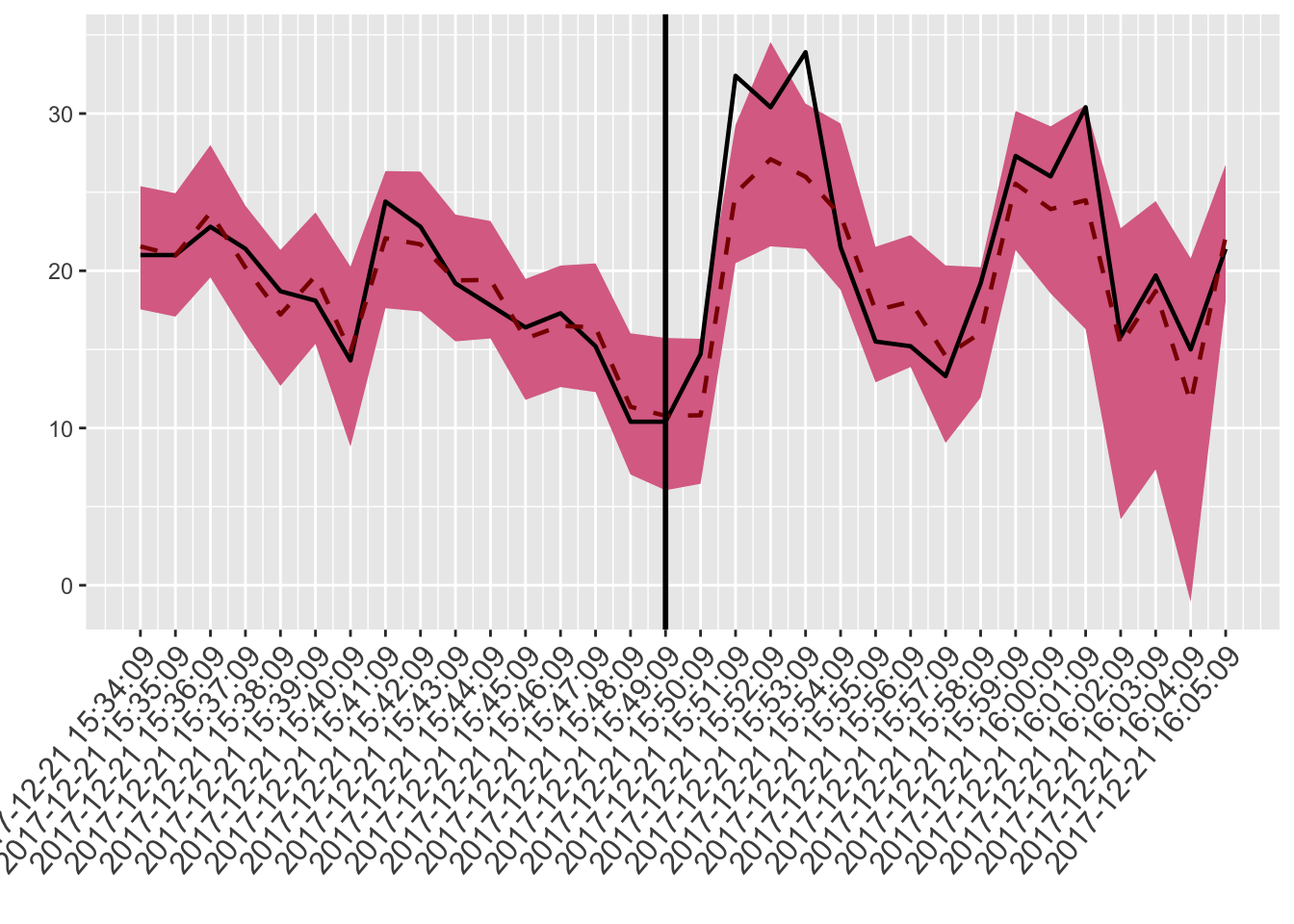
You may wonder why it uses reference and measurement instead of training and testing. In anomaly detection, espeically in telecommuncation field, performance reference period refers a period which serves a basis for defining anomaly, and performance measurement period refers the period during which performance parameters are measured.
If you hope to see the abstracted outcome, then:
summarise_session(.cbar)## session n_anomaly n_total rate
## 1 reference 0 16 0.000
## 2 measurement 2 16 0.125or you can just use print function as follows:
print(.cbar)## session n_anomaly n_total rate
## 1 reference 0 16 0.000
## 2 measurement 2 16 0.125or
summarise_session(.cbar)## session n_anomaly n_total rate
## 1 reference 0 16 0.000
## 2 measurement 2 16 0.125If you hope to see details of those anomalies:
summarise_anomaly(.cbar, .session = "measurement")## datetime session y point_pred lower_bound upper_bound
## 1 2017-12-21 15:50:09 measurement 14.7 10.80981 6.453536 15.67128
## 2 2017-12-21 15:51:09 measurement 32.4 24.94162 20.481840 29.27472
## 3 2017-12-21 15:52:09 measurement 30.4 27.09495 21.555414 34.54683
## 4 2017-12-21 15:53:09 measurement 33.9 25.98294 21.388805 30.63084
## 5 2017-12-21 15:54:09 measurement 21.5 23.51963 18.790273 29.36701
## 6 2017-12-21 15:55:09 measurement 15.5 17.47841 12.906749 21.52153
## 7 2017-12-21 15:56:09 measurement 15.2 18.03678 13.881706 22.26309
## 8 2017-12-21 15:57:09 measurement 13.3 14.58216 9.049250 20.34114
## 9 2017-12-21 15:58:09 measurement 19.2 16.05066 11.934944 20.22790
## 10 2017-12-21 15:59:09 measurement 27.3 25.53608 21.319480 30.16509
## 11 2017-12-21 16:00:09 measurement 26.0 23.92192 18.553984 29.18577
## 12 2017-12-21 16:01:09 measurement 30.4 24.48550 16.285601 30.51922
## 13 2017-12-21 16:02:09 measurement 15.8 15.29917 4.195908 22.70719
## 14 2017-12-21 16:03:09 measurement 19.7 18.70781 7.364142 24.43209
## 15 2017-12-21 16:04:09 measurement 15.0 11.63437 -1.049732 20.79486
## 16 2017-12-21 16:05:09 measurement 21.4 22.17463 18.028705 26.74785
## anomaly
## 1 FALSE
## 2 TRUE
## 3 FALSE
## 4 TRUE
## 5 FALSE
## 6 FALSE
## 7 FALSE
## 8 FALSE
## 9 FALSE
## 10 FALSE
## 11 FALSE
## 12 FALSE
## 13 FALSE
## 14 FALSE
## 15 FALSE
## 16 FALSEAnd if you rather want to check prediction performance:
summarise_pred_error(.cbar)## datetime session diff mape
## 1 2017-12-21 15:50:09 measurement 3.8901875 0.26463861
## 2 2017-12-21 15:51:09 measurement 7.4583765 0.23019680
## 3 2017-12-21 15:52:09 measurement 3.3050472 0.10871866
## 4 2017-12-21 15:53:09 measurement 7.9170636 0.23354170
## 5 2017-12-21 15:54:09 measurement 2.0196337 0.09393645
## 6 2017-12-21 15:55:09 measurement 1.9784081 0.12763923
## 7 2017-12-21 15:56:09 measurement 2.8367803 0.18663028
## 8 2017-12-21 15:57:09 measurement 1.2821648 0.09640337
## 9 2017-12-21 15:58:09 measurement 3.1493389 0.16402807
## 10 2017-12-21 15:59:09 measurement 1.7639188 0.06461241
## 11 2017-12-21 16:00:09 measurement 2.0780782 0.07992608
## 12 2017-12-21 16:01:09 measurement 5.9145010 0.19455595
## 13 2017-12-21 16:02:09 measurement 0.5008259 0.03169784
## 14 2017-12-21 16:03:09 measurement 0.9921852 0.05036473
## 15 2017-12-21 16:04:09 measurement 3.3656267 0.22437511
## 16 2017-12-21 16:05:09 measurement 0.7746257 0.03619746to visualise:
plot_error(.cbar, method = "mape")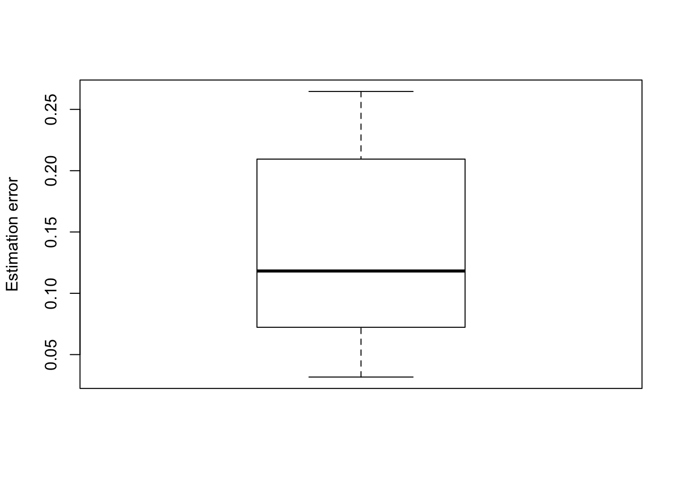
Structural analysis
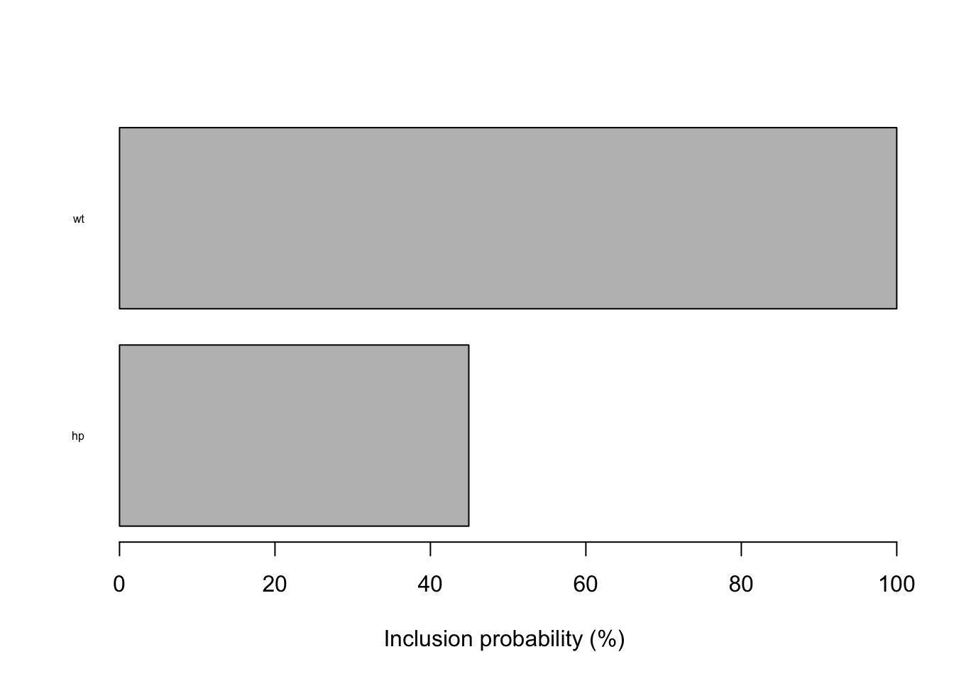
This Bayesian algorithm selects the best indicators, so we can make use of those selected indicators for structural analysis. Note that those indicators will be selected during the reference period.
To see those indicators:
summarise_incprob(.cbar)## hp wt
## 0.449398 1.000000to visualise:
plot_incprob(.cbar)